By DUY HUYNH in Programming — Oct 24, 2024

Building a Database From Scratch: Understanding LSM Trees and Storage Engines (Part 1)

Learn core database concepts by implementing a Python key-value store with crash recovery and efficient writes.

In this tutorial, we'll build a simple but functional database from scratch with Python. Through this hands-on project, we'll explore core database concepts like Write-Ahead Logging (WAL), Sorted String Tables (SSTables), Log-Structured Merge (LSM) trees, and other optimization techniques. By the end, you'll have a deeper understanding of how real databases work under the hood.

Why Build a Database?

Before diving into implementation, let's understand what a database is and why we're building one. Building a database from scratch is not just an educational exercise—it helps us understand the tradeoffs and decisions that go into database design, making us better at choosing and using databases in our own applications. Whether you're using MongoDB, PostgreSQL, or any other database, the concepts we'll explore form the foundation of their implementations.

A database is like a digital filing cabinet that helps us:

Store data persistently (meaning it survives even when your computer restarts)
Find data quickly when we need it
Keep data organized and consistent
Handle multiple users accessing data at the same time
Recover from crashes without losing information

In this tutorial, we'll build a simple database that stores key-value pairs. Think of it like a Python dictionary that saves to disk. For example:

You might wonder: "Why not just save a Python dictionary to a file?" Let's start there to understand the problems we'll need to solve.

Let's break down what this code does:

__init__(self, filename):
- Creates a new database using a file to store data
- filename is where we'll save our data
- self.data is our in-memory dictionary
_load(self):
- Reads saved data from disk when we start
- Uses Python's pickle module to convert saved bytes back into Python objects
- The underscore (_) means it's an internal method not meant to be called directly
_save(self):
- Writes all data to disk
- Uses pickle to convert Python objects into bytes
- Called every time we change data
set(self, key, value) and get(self, key):
- Works like a dictionary's [] operator
- set saves to disk immediately
- get returns None if key doesn't exist

This simple implementation has several problems:

Crash risk:

Performance issue:

Memory limitation:

Concurrency issue:

Write-Ahead Logging (WAL) - Making It Durable

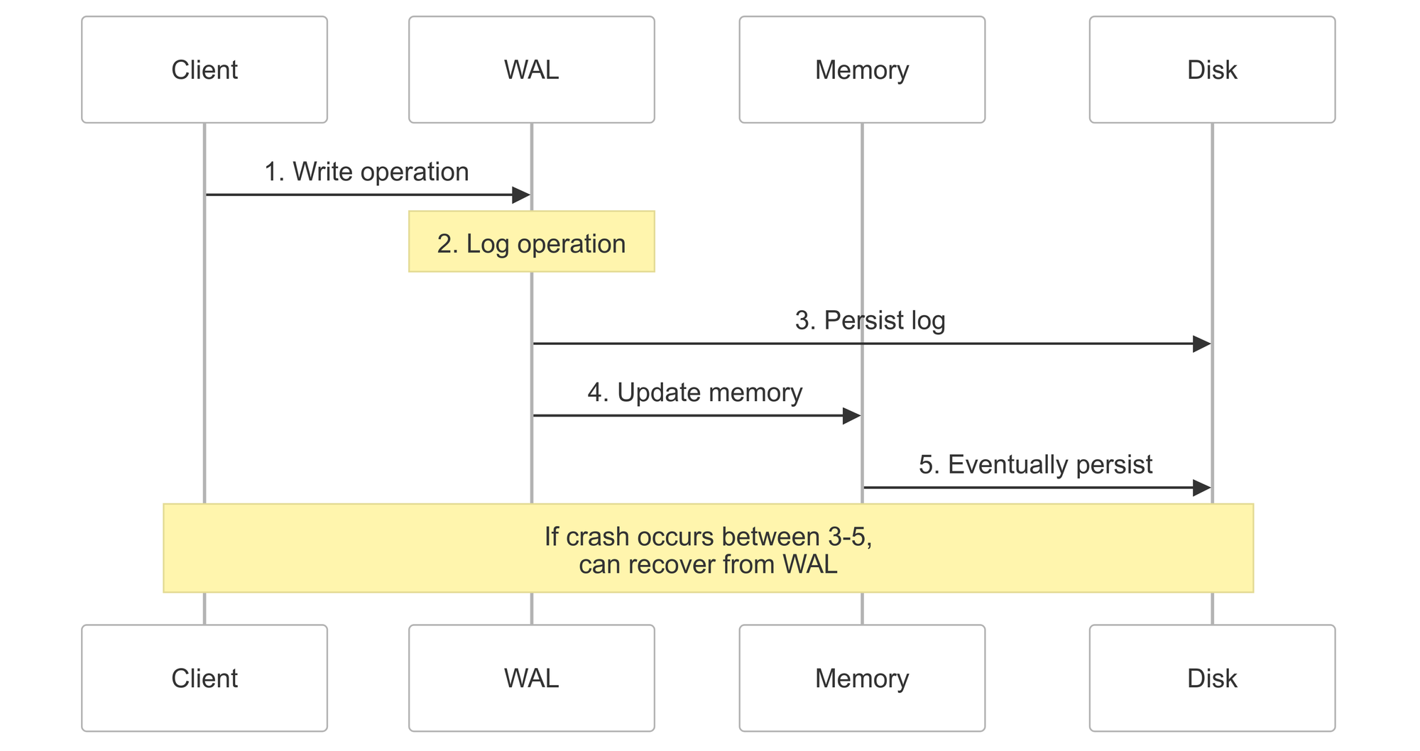
First, to ensure data persistence and recovery capabilities, we will use Write-Ahead Logging. Write-Ahead Logging is like keeping a diary of everything you're going to do before you do it. If something goes wrong halfway through, you can look at your diary and finish the job. WAL is a reliability mechanism that records all changes before they are applied to the database.

Example:

# WAL entries are like diary entries:
Entry 1: "At 2024-03-20 14:30:15, set user:1 to {"name": "Alice"}"
Entry 2: "At 2024-03-20 14:30:16, set user:2 to {"name": "Bob"}"
Entry 3: "At 2024-03-20 14:30:17, delete user:1"

This safety-first approach ensures that even if our database crashes after logging but before completing the operation, we can recover by replaying our WAL entries.

Let's understand what each part means:

timestamp: When the operation happened

# Example timestamp
"2024-03-20T14:30:15.123456"  # ISO format: readable and sortable

operation: What we're doing

# Example operations
{"operation": "set", "key": "user:1", "value": {"name": "Alice"}}
{"operation": "delete", "key": "user:1", "value": null}

serialize: Converts to string for storage

# Instead of binary pickle format, we use JSON for readability:
{
    "timestamp": "2024-03-20T14:30:15.123456",
    "operation": "set",
    "key": "user:1",
    "value": {"name": "Alice"}
}

The WAL Store Implementation

In this implementation, we keep track of 2 files: the data_file and wal_file. The data_file serves as our permanent storage where we save all data periodically (like a database backup), while the wal_file acts as our transaction log where we record every operation before executing it (like a diary of changes).

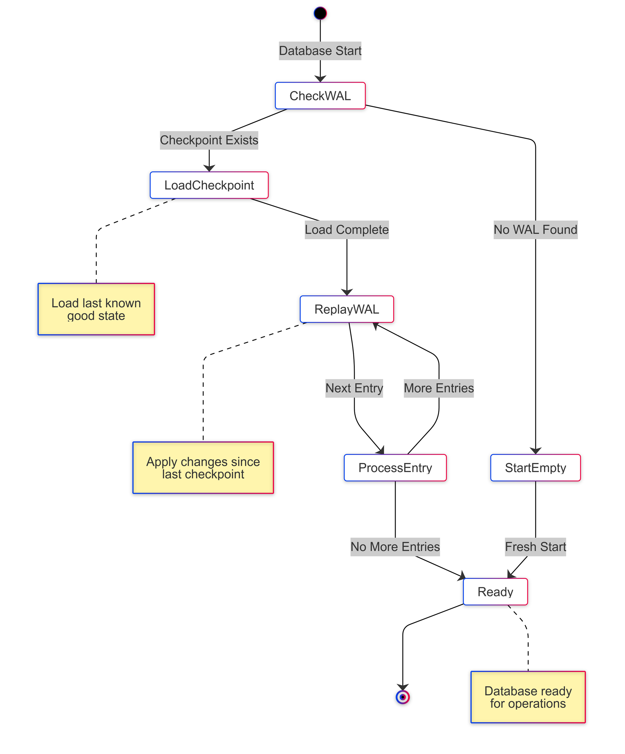
The recovery process works like this:

First loads the last saved state from data_file
Then replays all operations from the WAL file
Handles both 'set' and 'delete' operations

Example of recovery sequence:

# data_file contains:
{"user:1": {"name": "Alice"}}

# wal_file contains:
{"operation": "set", "key": "user:2", "value": {"name": "Bob"}}
{"operation": "delete", "key": "user:1"}

# After recovery, self.data contains:
{"user:2": {"name": "Bob"}}

Another important method of this implementation is checkpoint. It creates a permanent snapshot of current state. Here is an example of checkpointing process:

1. Current state: 
   data_file: {"user:1": {"name": "Alice"}}
   wal_file: [set user:2 {"name": "Bob"}]

2. During checkpoint:
   data_file: {"user:1": {"name": "Alice"}}
   data_file.tmp: {"user:1": {"name": "Alice"}, "user:2": {"name": "Bob"}}
   wal_file: [set user:2 {"name": "Bob"}]

3. After checkpoint:
   data_file: {"user:1": {"name": "Alice"}, "user:2": {"name": "Bob"}}
   wal_file: []  # Empty

Memory Tables - Making It Fast

MemTables serve as our database's fast write path, providing quick access to recently written data. They maintain sorted order in memory, enabling efficient reads and range queries while preparing data for eventual persistent storage. You can think of a MemTable like a sorting tray on your desk:

New items go here first (fast!)
Since all items are sorted, the search operation is fast using binary search for both single key queries and range queries (binary search cuts the search space in half with each step, giving us O(log n) performance instead of having to check every item)
When it gets full, you file them away properly (in SSTables)

Let's see how the memtable stays sorted:

While our implementation uses a simple sorted list with binary search, production databases like LevelDB and RocksDB typically use more sophisticated data structures like Red-Black trees or Skip Lists. We used a simpler approach here to focus on the core concepts, but keep in mind that real databases need these optimizations for better performance.

Sorted String Tables (SSTables) - Making It Scale

While MemTables provide fast writes, they can't grow indefinitely. We need a way to persist them to disk efficiently. Since our memory is limited, when the MemTable gets full, we need to save it to disk. We use SSTables for this. SSTables (Sorted String Tables) are like sorted, immutable folders of data:

File format explanation:

File layout:
[size1][entry1][size2][entry2]...

Example:
[0x00000020][{"key": "apple", "value": 1}][0x00000024][{"key": "banana", "value": 4}]...

Putting It All Together - The LSM Tree

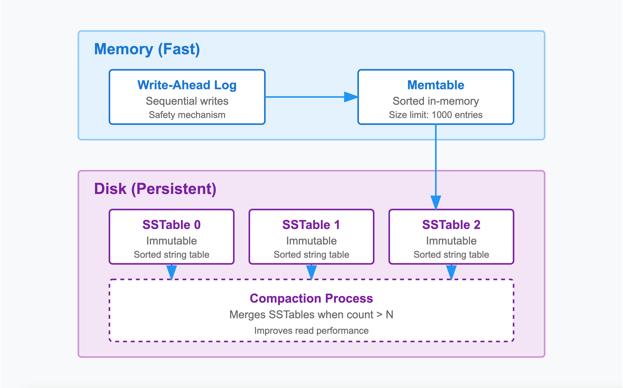
Now we'll combine everything we've learned (WAL, MemTable, and SSTables) into a simplified version of a Log-Structured Merge Tree (LSM Tree). While a true LSM tree uses multiple levels, we'll start with a basic flat structure in Part 1 and upgrade to a proper leveled implementation in Part 2 of this series.

Imagine you're organizing papers in an office:

New papers go into your inbox (MemTable)
- This is like the fast "write path" of the database
- Papers can be added quickly without worrying about organization yet
- The inbox is kept in memory for quick access
When inbox is full, you sort them and put in a folder (SSTable)
- The papers are now sorted and stored efficiently
- Once in a folder, these papers never change (immutable)
- Each folder has its own index for quick lookups
When you have too many folders, you merge them (Compaction)
- In our Part 1 implementation, we'll simply merge all folders into one
- This is a simplified approach compared to real databases. While functional, it's not as efficient as proper leveled merging

Here's how we implement our simplified version:

Simple Database Architecture

To ensuring thread safety in our database, we uses locks to prevent multiple threads from causing problems:

# Example of why we need locks:
# Without locks:
Thread 1: reads data["x"] = 5
Thread 2: reads data["x"] = 5
Thread 1: writes data["x"] = 6
Thread 2: writes data["x"] = 7  # Last write wins, first update lost!

# With locks:
Thread 1: acquires lock
Thread 1: reads data["x"] = 5
Thread 1: writes data["x"] = 6
Thread 1: releases lock
Thread 2: acquires lock
Thread 2: reads data["x"] = 6
Thread 2: writes data["x"] = 7
Thread 2: releases lock

Writing Data

Let's see how writing data works step by step:

Example of how data flows:

# Starting state:
memtable: empty
sstables: []

# After db.set("user:1", {"name": "Alice"})
memtable: [("user:1", {"name": "Alice"})]
sstables: []

# After 1000 more sets (memtable full)...
memtable: empty
sstables: [sstable_0.db]  # Contains sorted data

# After 1000 more sets...
memtable: empty
sstables: [sstable_0.db, sstable_1.db]

Reading Data

Reading needs to check multiple places, newest to oldest:

Example of reading:

# Database state:
memtable: [("user:3", {"name": "Charlie"})]
sstables: [
    sstable_0.db: [("user:1", {"name": "Alice"})],
    sstable_1.db: [("user:2", {"name": "Bob"})]
]

# Reading "user:3" -> Finds it in memtable
# Reading "user:1" -> Checks memtable, then finds in sstable_0.db
# Reading "user:4" -> Checks everywhere, returns None

Compaction: Keeping Things Tidy

# Before compaction:
sstables: [
    sstable_0.db: [("apple", 1), ("banana", 2)],
    sstable_1.db: [("banana", 3), ("cherry", 4)],
    sstable_2.db: [("apple", 5), ("date", 6)]
]

# After compaction:
sstables: [
    sstable_compacted.db: [
        ("apple", 5),    # Latest value wins
        ("banana", 3),   # Latest value wins
        ("cherry", 4),
        ("date", 6)
    ]
]

We also need other methods, such as deleting and closing the database instance:

Here's how to use what we've built:

Our implementation provides the following complexity guarantees:

Operation	Complexity	Notes
Write	$$O(\log{n})$$	Binary search in MemTable
Read	$$O(\log{n})$$	Per SSTable searched
Range Query	$$O(k\log{n})$$	k = range size
Compaction	$$O(n\log{n})$$	Full merge sort

Testing Our Database

Let's put our database through some basic tests to understand its behavior:

Running these tests helps ensure our database is working as expected!

Conclusion

In this first part of our journey to build a database from scratch, we've implemented a basic but functional key-value store with several important database concepts:

Write-Ahead Logging (WAL) for durability and crash recovery
MemTable for fast in-memory operations with sorted data
Sorted String Tables (SSTables) for efficient disk storage
Log-Structured Merge (LSM) Tree to tie everything together

Our implementation can handle basic operations like setting values, retrieving them, and performing range queries while maintaining data consistency and surviving crashes. By converting random writes into sequential ones, LSM Trees excel at quickly ingesting large amounts of data. This is why databases like RocksDB (Facebook), Apache Cassandra (Netflix, Instagram), and LevelDB (Google) use LSM Trees for their storage engines. In contrast, traditional B-Tree structures (used by PostgreSQL and MySQL) offer better read performance but may struggle with heavy write loads. We’ll explore B-Tree implementations in future posts to better understand these trade-offs.

Current Limitations

While our database works, it has several limitations that we'll address in the coming parts:

Storage and Performance:

Simple list of SSTables instead of a leveled structure
Inefficient compaction that merges all tables at once
No way to skip unnecessary SSTable reads, scan all table for a query is inefficient.

Concurrency:

Basic locking that locks the entire operation
No support for transactions across multiple operations
Compaction process blocks all other operations

In Part 2, we'll tackle some of these limitations by implementing level-based compaction, bloom filters for faster lookups, and basic transaction support. Stay tuned

The complete source code for this tutorial is available on Github. I encourage you to experiment with the code, try different optimizations, and share your findings in the comments below.